
Inertial Measurement Unit (IMU) – An Introduction
Share:
Published on:
Table of Contents
- Introduction
- The Technology Behind IMU Sensors
- IMU Calibration
- Interpreting Inertial Measurement Unit Specifications
Introduction
This article explains the concepts of inertial measurement and the technology behind motion sensing and measurement.
The measurement of motion, specifically, acceleration, rotation and velocity, is essential to understanding the orientation of an object. It is also broadly applicable to many applications; for example, production line machines, robotic devices, vehicles, autonomous systems, gimbals, machine tools, and even robotic prosthetics.
Advancements in technology, manufacturing techniques, miniaturization, and computerized processing have greatly simplified the production of motion sensing devices used in IMUs (particularly those using MEMS technology).
An IMU (sometimes referred to as an inertial reference unit [IRU] or motion reference unit [MRU]) is typically an electromechanical or solid-state device that contains an array of sensors that are able to measure motion. That is, to detect linear acceleration (the rate of change in velocity) and angular rate (change in angular velocity) in about the X, Y and Z axes and provide data about that motion
The IMU is able to measure motion by converting the detected inertia, which are forces created due to an object’s resistance to changing direction, into output data that describes the motion of the object. This data will be used by some other system, for example, to control a vehicle. The output of an IMU is typically the raw sensor data from:
- accelerometers (linear acceleration measurements along each axis)
- gyroscopes (rotational rates/angular velocity measurements around each axis)
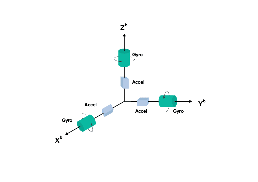
Image depicting the accelerometers and gyroscopes in the three axes of movement. Each accelerometer and gyroscope is positioned at 90 ° to the others (orthogonally). Accelerometers measure motion along each axis and each gyroscope measures angular velocity around each axis.
IMU Sensor Data
Recorded IMU signals or sensor from the IMU is processed by additional devices or systems that provide a frame of reference to which the IMU data is applied. An aerial vehicle, using the Earth as the reference frame, for example, will fuse IMU data into its navigation system to determine vehicle heading and position with reference to the Earth – geographical location and heading relative to north. The raw IMU sensor information may be sufficient for determining orientation (for example, am I pointing up?) and movement (for example, am I moving?) and be used in more complex calculations, such as when dead-reckoning. Typical applications include:
- Motion tracking
- Vibration monitoring
- Consumer electronics – phones
- Pointing applications – camera and antenna positioning
Differences Between the Inertial Measurement Unit (IMU) and Attitude and Heading Reference System (AHRS)
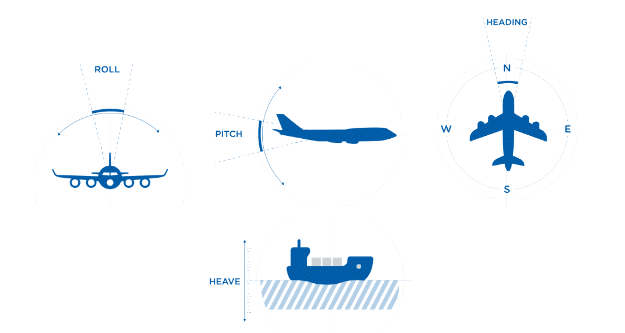
The IMU is often confused with AHRS (attitude, heading and reference system) devices. The main difference being that an AHRS will provide orientation/heading data in addition to motion data.
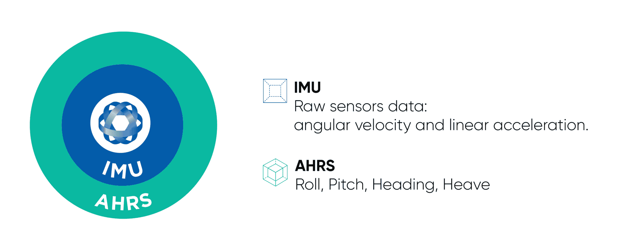
An AHRS contains an IMU for motion sensing; however, it uses additional sensor fusion techniques and on-board processing to combine the raw sensor outputs to determine an accurate roll, pitch, heading, and heave in its output data.
The Technology Behind IMU Sensors
The accelerometers, gyroscopes (and sometimes magnetometers) within inertial measurement units are generically known as “inertial sensors”.
MEMS Inertial Sensors
The most common technology used in the production of inertial sensors today is MEMS – micro-electromechanical systems. MEMS are extremely tiny devices (down to micrometers in size) that are a combination of electrical and mechanical elements made from various materials (such as silicon, polymers, metal) that are designed to provide a specific function. For example, a MEMS accelerometer to measure linear acceleration. MEMS components vary in complexity from simple switches to extremely intricate electromechanical systems that have multiple integrated sensors and microelectronics.
Sensor data processing takes into account the gravitational effects of the Earth to provide outputs that are accurately representative of actual movement in free space. To describe the gravitational effect, imagine an IMU in free fall; it will measure a zero vertical acceleration because the entire unit is accelerating at the same rate as the gravitational pull of the Earth. If we stop the IMU, so it’s floating in free space, it would measure a vertical acceleration of -9.81 m/s2 although to us it appears stationary – this gravitational acceleration has to be removed from the sensor output. This means that when floating in free space, vertical acceleration is 0 m/s2.
Advantages of MEMS Technology
- Extremely small size and weight components – This means that the sensors can be mounted on small printed circuit boards and housed in small casings. The small form factor makes MEMS very well suited to applications that are sensitive to payload size and weight.
- Very low power consumption – MEMS sensors consume exceedingly small amounts of power, making them excellent for battery-powered applications.
- More cost-effective – MEMS silicon etching, micro-machining and PCB mounting are well suited to mass production, making MEMS devices relatively inexpensive.
- Reliability – MEMS components and the materials and construction techniques make them an extremely reliable sensor type that can offer very long service lifetimes.
- Quick gyroscopic initialization – MEMS gyroscopes are able to “settle” faster than mechanical and optical sensor types. This makes the sensor available for use earlier following start-up.
- Improving technology – MEMS sensors are extremely widely used and this is leading to continued development and refinement to increase accuracy, further miniaturize, and lower costs. Currently, there are MEMS gyroscopes that are capable of matching the gyroscopic performance of some fibre-optic gyroscopes (FOGs).
MEMS and FOG Gyroscopes – A Brief Comparison
For applications requiring extremely high-accuracy rotational measurement and heading, other gyroscope technologies are available. These are typically used in applications that are not able to rely on magnetic heading and may not be able to acquire GNSS data for assistance. For example, subsea applications where there is no GNSS reception and magnetic heading is not accurate enough or is disrupted by magnetic interference from surrounding ferrous materials or environmental conditions.
In the above mentioned scenario, a fibre-optic gyroscope (FOG), may provide the necessary gyroscopic performance – ultra-high accuracy and precision, low drift and low bias instability, and immunity to magnetic interference. The benefits of FOG technology are offset somewhat by being, in comparison to a typical MEMS IMU, many times larger, notably heavy, and very much more expensive. In real terms, this has limited the market and applications that a FOG is not only suited to, but makes sense to use in, and that the necessary investment required is acceptable.
The size/weight/cost disadvantages that limits the use of FOG gyroscopes has helped compound the assurgency of MEMS as a viable alternative technology with excellent physical and performance characteristics. The affordability and accessibility of MEMS IMU technology has made it applicable to a much greater user base and range of applications, including being a key augmenting technology in the robotics and autonomous system industries.
As an example, the Motus MEMS IMU from Advanced Navigation offers compact size, minimal weight, lower power consumption and cost (SWaP-C), whilst remaining capable of very high accuracy gyroscopic performance. Motus weighs 26 g (~1 oz), requires ~16 cm3 (~1 “3) of volume, and draws 1.4 W. The following is a performance comparison of Advanced Navigation Motus MEMS IMU and Boreas D90 digital FOG INS.
| Motus | Boreas D90 | |
| Roll and Pitch | 0.05 ° | 0.005 ° |
| Heading | 0.8 ° (magnetic) | 0.01 ° |
| Bias Instability | 0.2 °/hr | 0.001 °/hr |
In the above comparison, the choice of IMU will depend on a combination of factors that are determined by how much accuracy you need, how suitable is each available option for the actual application, and how much you want to spend. Although the Boreas is, hands down, a more accurate and, therefore, more costly device; on the physical side of things, it weighs 2500 g (~88 oz), requires 2600 cm3 (~158 “3) of volume and draws 12 W. It is easy to see major differences in performance and size, weight, power consumption and cost (SWaP-C) between the two.
To put the above into context, to use a FOG in a small-scale UAV application may mean using a drone with a higher payload capacity, which is usually larger to accommodate the necessary motors, batteries and payload. In this case, a MEMS-based IMU INS with magnetometer heading is well suited as it presents minimal payload, particularly if available in OEM form, consumes little power and can provide accuracy that makes MEMS inertial sensing applicable to a broad range of UAV-based applications, such as LiDAR surveying and photogrammetry.
IMU Sensors
Accelerometers
Accelerometers are motion sensors that measure linear acceleration/rate of change in velocity of an object, relative to a local inertial reference frame. As a concept, the accelerometer consists of a proof mass attached to its reference frame by mechanical springs. The springs allow movement of the proof mass along what is known as the sensitivity axis. Measuring the displacement of the proof mass (that is, how far the mass has moved from its previous position) allows computation of the applied acceleration.
Measurement of the displacement is performed through electrical capacitance. The sensor will have several differential capacitors. These are electrodes that are fixed in place either side of the proof mass. The proof mass will have extension arms or “fingers” that protrude into the space between the differential capacitor electrodes. At a standstill, the fingers are centered between the electrodes and a known capacitance is produced to represent zero acceleration. During an acceleration event, the proof mass moves – this is because it is sprung and so will accelerate at a different rate to the rest of the sensor (the reference frame). As a result, the fingers move closer to one electrode, creating a change in capacitance from which acceleration can be derived.
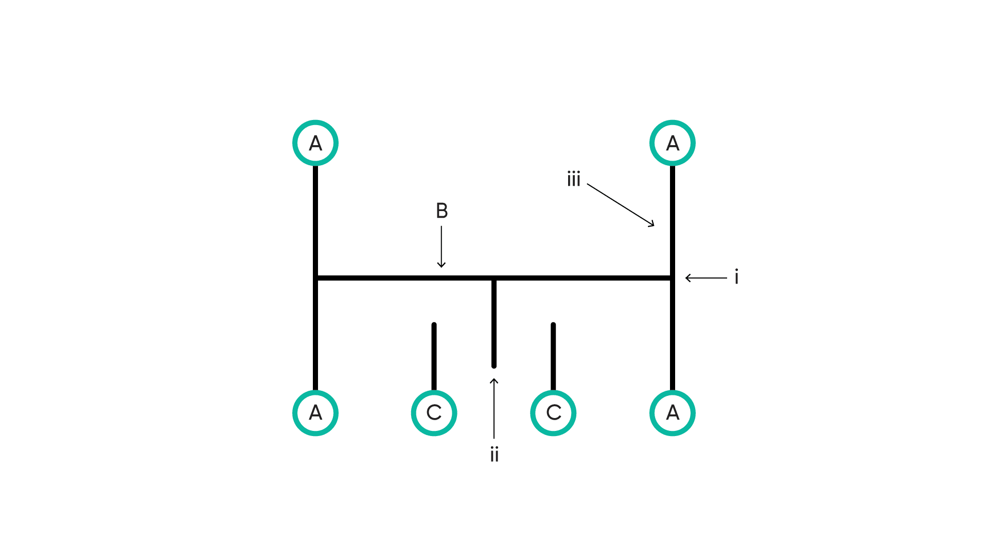
Image depicts the operation of a simple MEMS accelerometer. The anchors (A) hold the proof mass (B) in position. The proof mass consists of a centre section (i), with several protruding fingers (ii). The sections of the proof mass between the centre section and anchors act as the springs (iii). The fixed electrodes (C) make up the differential capacitors, with a protruding finger from the proof mass between the capacitor electrodes. When the accelerometer is at rest or is traveling at a fixed velocity (zero acceleration), the fingers are in the centre position between the electrodes, as shown.
In the above animation, the first sequence shows the accelerometer stationary. It is then accelerated to the right. The resistance to acceleration (the inertia) of the proof mass causes it to want to remain stationary, and so accelerates at a different rate to the reference frame, causing it to pull to the left on the springs. The change in capacitance of the differential capacitors represents the amount of acceleration being sensed – the closer the finger is to the left-side electrode, the greater the acceleration is to the right.
In the second sequence, the force causing the acceleration to the right is stopped. This immediately creates a decelerative force due to friction, for example. The proof mass moves now toward the right-side electrode, from which a negative acceleration value is computed. Eventually, enough force is reapplied that the accelerometer is traveling at a constant velocity, so the fingers are in the centre of the differential capacitor electrodes.
In the final sequence, the accelerometer is brought from a constant velocity down to zero velocity, under heavy deceleration, then is again stationary.
Open-loop and closed-loop accelerometers
There are two main classes of accelerometer sensor – open-loop, and closed-loop. Open-loop sensors have a proof mass that displaces under acceleration, with the displacement measured to calculate the applied acceleration (as described above). These sensors are less complex and cost less to manufacture.
A closed-loop accelerometer is a device that typically maintains its proof mass in a fixed position and measures the current or power needed to maintain it in that position – in other words, the power required to cancel the accelerative force. A significant difference between the two is that the closed-loop system is able to provide feedback about its state, which allows the sensor to be self-regulating and, as a result, possibly more accurate. Several other methods of measuring proof mass displacement are in use, including piezoresistive, piezoelectric, and tuneling current measurement.
MEMS accelerometers are designed specifically for an intended maximum permissible acceleration. These are necessary to achieve the required measurement resolution and dynamic range.
Gyroscopes
Angular rate sensors, commonly known as gyroscopes, indicate acceleration (rate of rotation) about an axis. While multiple techniques for measuring angular acceleration exist, the most common method uses the Coriolis effect. To visualize the Coriolis effect, imagine a circular platform rotating in a clockwise direction, with a vehicle at its centre. The vehicle begins moving in a northward direction. As the vehicle moves further from the centre, the radial velocity of the platform increases, which causes the vehicle to effectively follow a reducing radius arc, seemingly to the west – this change in direction is the Coriolis effect. To maintain a northward course, the vehicle must cancel the Coriolis effect by applying equal and opposite acceleration – this is Coriolis acceleration.
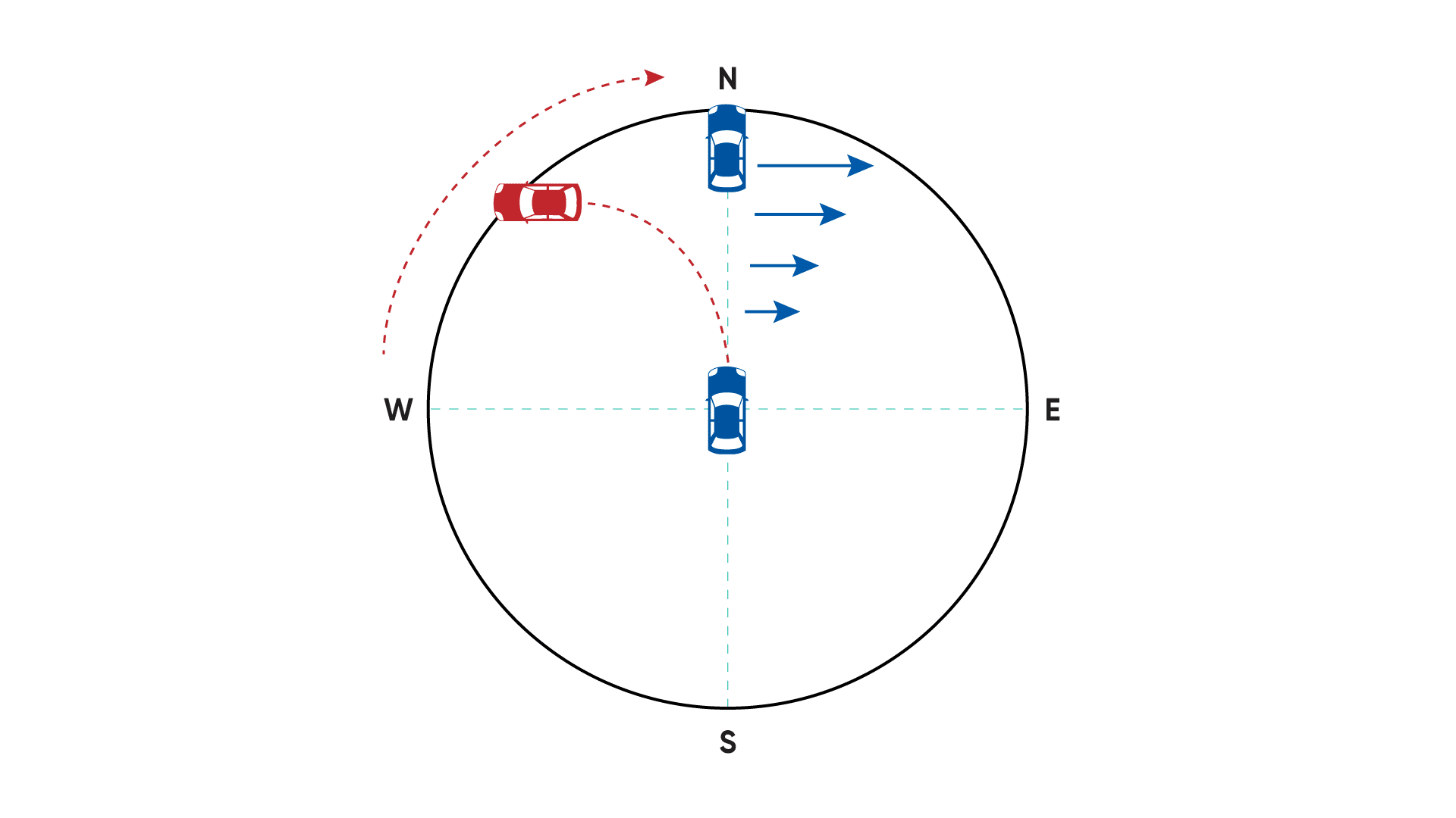
When viewed from above, a vehicle moving northward towards the outer edge of a rotating platform will reach the edge of the platform in a north-westerly position due to the increasing radial speed of the platform beneath the vehicle – the Coriolis effect (dashed red line). To maintain a northward course, the vehicle will need to accelerate toward the east in proportion to the Coriolis effect – this is Coriolis acceleration (blue arrows). The faster the platform rotates, the more acute the Coriolis effect becomes.
Using the Earth as the frame of reference, the Coriolis effect is the apparent deflection caused to a moving object due to simultaneous rotation of the Earth and relative latitude. For example, when launching a rocket northward from the equator – in the time it takes for the rocket to land, the Earth has rotated an amount eastward. This means that the rocket travels, relative to the Earth’s surface, in a left curving arc, and lands due west of its intended landing point (although it has travelled straight). As you move toward the poles and latitude increases, so increases the Coriolis effect due to the reducing circumference of the Earth.
In a typical Coriolis MEMS gyroscope, a resonating proof mass is attached to its reference frame by mechanical springs. This reference frame is attached to an outer reference frame and isolated by mechanical springs. The proof mass is made to vibrate along a particular axis – this is known as the drive axis. When the gyroscope is rotated, the Coriolis effect induces a secondary vibration along the axis perpendicular to the drive axis – this is known as the sense axis. As with many MEMS accelerometer sensors, the measurement is derived through electrical capacitance. Rotation causes a change in the output of the differential capacitance between the inner and outer frames of reference. As the rate of rotation increases, so does the displacement of the proof mass, producing a signal proportional to the Coriolis force / sensed rotation.
Image depicts the operation of a simple MEMS Coriolis gyroscope. The springs (A) hold the proof mass (B) in position within the inner frame of reference (C). The inner reference frame is isolated from the outer frame of reference (D) also using springs (E). The inner frame of reference has several protruding fingers (i). The fixed electrodes (ii) make up the differential capacitors, with a protruding finger from the inner frame of reference between the capacitor electrodes. The gyroscope may be placed anywhere and at any angle on the rotating object , however, its sense axis must be parallel to the axis of rotation.
Magnetometers
A magnetometer is used to detect and measure the strength and direction of the Earth’s magnetic fields in order to determine heading. Magnetic heading derives north-related direction using a combination of the Earth’s magnetic field strength. Three magnetometers measure the magnetic field strength to provide a three-dimensional orientation, with respect to magnetic north. Note that magnetic north is not the same as “true” (geographical) north, which is the axis that the Earth revolves around.
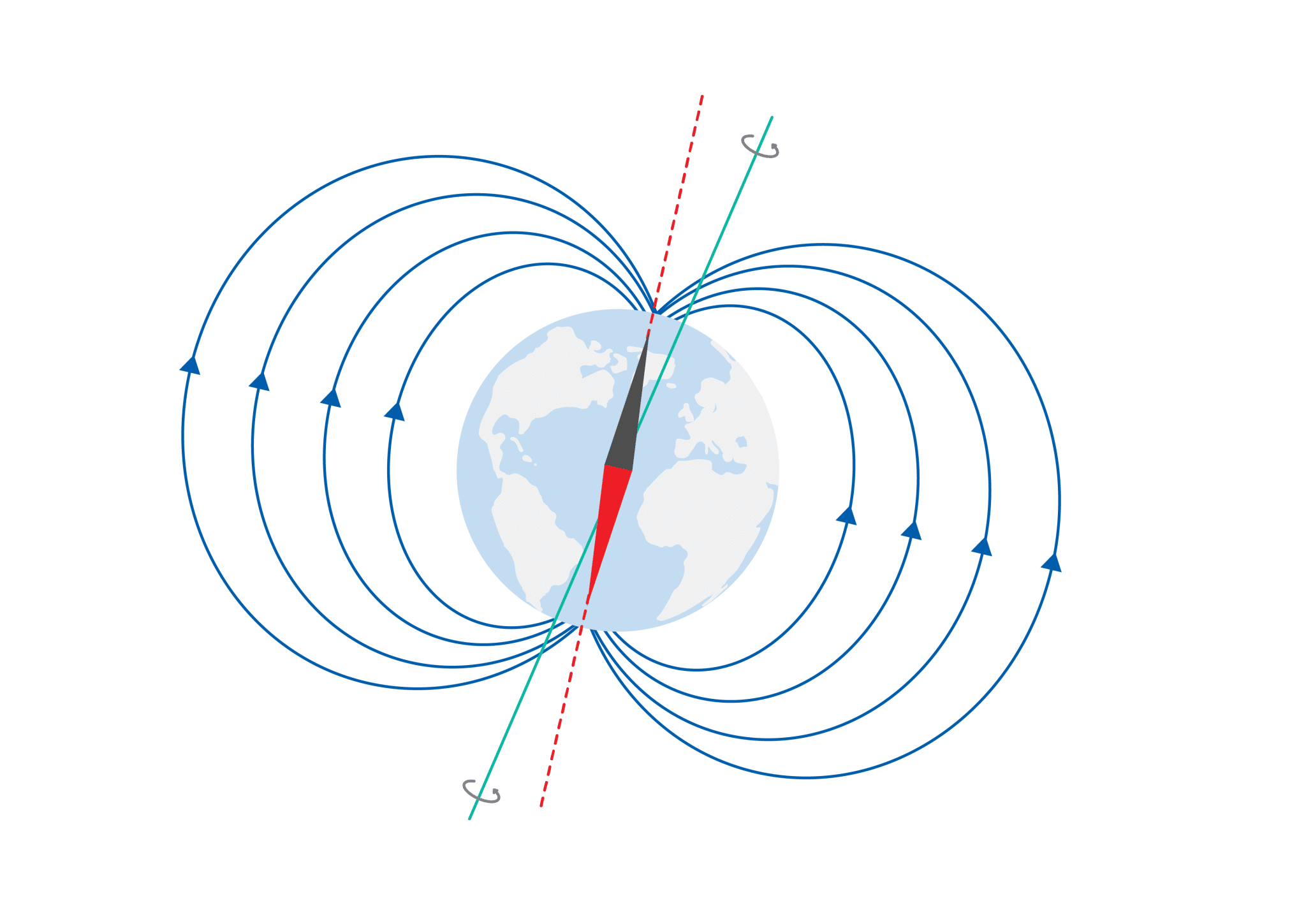
The red axis depicts “magnetic north” as it is aligned with the Earth’s magnetic fields. The blue axis represents “true north” as it is the actual axis that the Earth spins around.
Two predominant magnetometer technologies are magneto-resistive and Hall-effect. Hall-effect sensors measure the difference in electrical potential between two sides of a current-carrying strip when the strip is in the presence of magnetic fields perpendicular to the direction of the current.
Magneto-resistive sensors use permalloys with magnetic domains aligned in the same direction. A change in the Earth’s magnetic field alters the magnetic alignment within the permalloy, altering its resistance. This variation can be measured and used to calculate changes in heading.
Magnetometers are highly sensitive, which makes them susceptible to electromagnetic interference that can affect accuracy. This means that the magnetometers must be calibrated during commissioning.
To summarize typical major advantages to the above mentioned sensor types:
| Magneto-resistive | Hall-effect |
| Higher sensitivity | Distinguishes between north and south magnetic poles |
| Lower noise | Less prone to interference |
| Higher angular sensitivity | Greater angular measurement (360°) |
Pressure Sensors
Pressure sensors are used to measure external pressure on the IMU. For example, a water pressure sensor for determining depth in underwater applications, and an air pressure sensor (barometer) for determining altitude. The higher the altitude, the lower the air pressure; the greater the depth, the higher the water pressure. Two primary methods of determining pressure are through piezoresistance or capacitance. Both use a diaphragm that deflects when under pressure – the deflection is used to create a measurable value.
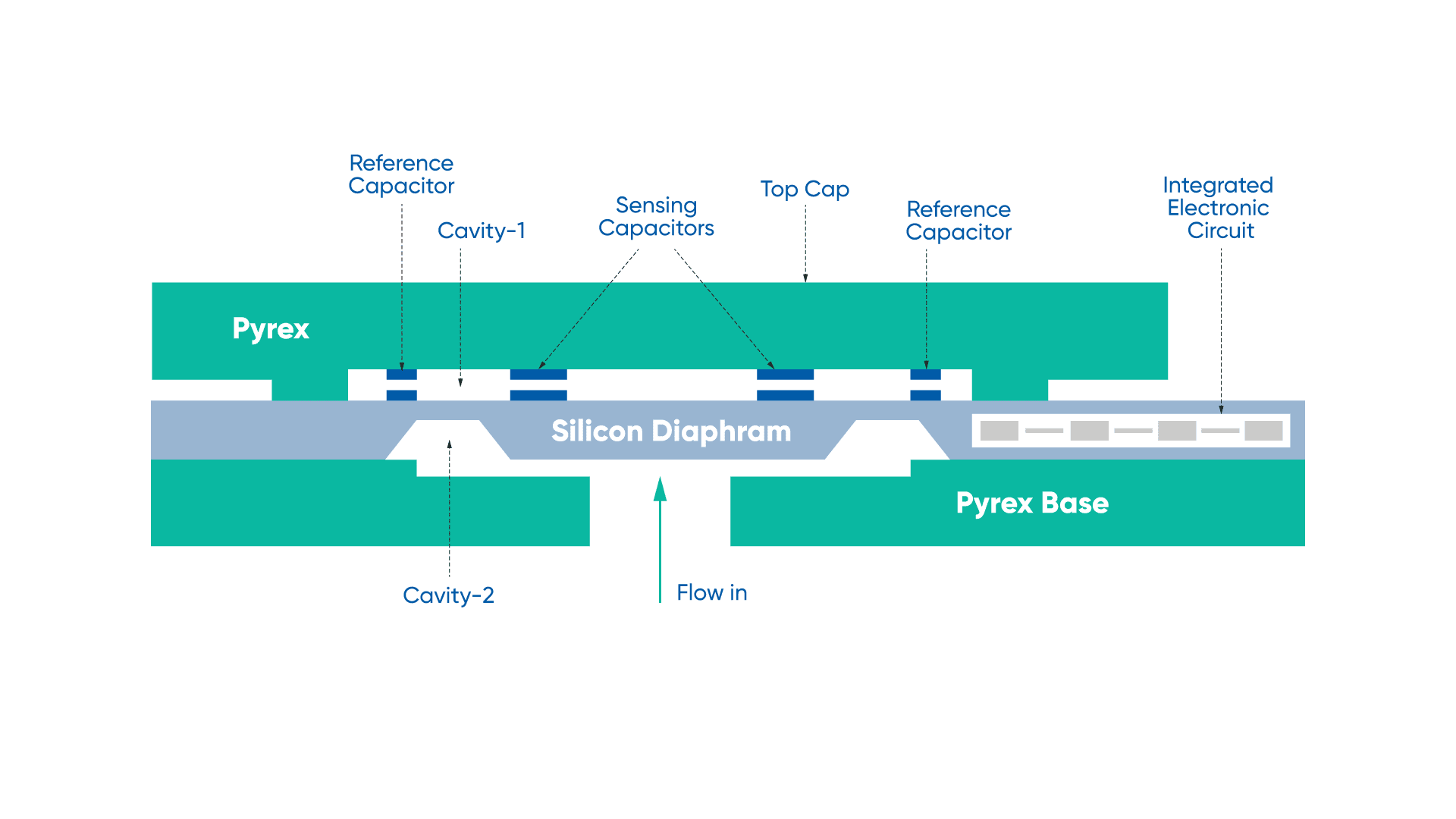
Changes of pressure in the in-flow cavity causes the diaphragm to deflect. Differential capacitors in the sensing cavity change capacitance depending on the distance between the capacitor electrodes. As pressure increases, the electrodes on the diaphragm move closer to the electrodes on the sensing cavity wall.
A capacitive pressure sensor will have conductive layers deposited on the underside of the diaphragm to create the capacitor. When the pressure increases, for example, the diaphragm is pressurized and will deflect, with the change in spacing between the diaphragm and the electrodes, altering the measured capacitance.
The piezo-resistive method etches conductive elements directly onto the surface of the diaphragm, creating two parallel sets of known resistances that, through computation, can accurately determine an unknown resistance. This is known as a Wheatstone bridge network. As the diaphragm deflects due to changes in pressure, there is an undetermined change in resistance (the unknown variable). The Wheatstone bridge circuit measures the resistance, which is representative of pressure against the diaphragm.
To summarize typical major advantages to the above mentioned sensor types:
| Capacitive | Piezo-resistive |
| Longer term stability | Simpler calibration |
| Lower power consumption Higher accuracy and lower total error band Greater resistance to over-pressure | Lower cost |
Fibre-Optic Gyroscopes
Fibre-optic gyroscopes (FOG) are the preeminent technology for IMUs that must provide ultra-high accuracy and precision, low drift and low bias instability. That is, gyroscopic performance that is beyond the performance limitations of MEMS devices. Additionally, many FOGs are capable of gyrocompassing, which is to find true north based on rotation of the Earth, unaided by magnetometers or GNSS. This makes FOGs immune to magnetic interference and, therefore, a good choice for applications where magnetic heading is not an option.
A FOG uses an optical phenomena called the Sagnac effect to determine the rotational rate of the unit. A FOG has three coils of optical fibre placed orthogonally (at 90 ° to one another) – one each for the X, Y and Z axes. A laser is used to send a light beam simultaneously in opposing directions through each coil winding. Another optical gyroscope technology is the ring laser gyroscope (RLG). This type device uses mirrors to control the path of the laser light instead of coils of optical fibre.
When the light exits the coil, the waveforms are combined (interfered) and the resultant waveform examined. If a rotation has occurred, the effective time required for the light in one direction to travel the coil will differ to that of the other (think of this as a race track with two equally fast cars traveling in opposite directions, with the actual track and finish line moving beneath the cars). If there is any phase shift between the two, this will be evident in the combined waveform. A fibre-optic gyroscope uses the phase shift to calculate rotation to a high degree of accuracy.
In the graphic, the FOG is rotating about the Z-axis. During rotation, the phase shift of the light can be seen as a difference in arrival time of the two light beams at the optical receiver. Phase shift in the light occurs only during rotation; once the rotation stops, the light will again be in phase. Note that this is for illustrative purposes only and not necessarily a depiction of the actual technology.
FOG requires no moving parts, does not rely on inertial resistance, and also generates very little electrical noise to hamper its accuracy. In other words, inherent lower drift characteristics and resistance to vibration, acceleration and shock induced errors. Note that a FOG that is also an INS will typically use high-end MEMS sensors for non-gyroscopic sensing.
IMU Calibration
Calibration is critical to ensuring that the output from sensors is accurate and repeatable within the specified operating conditions. That is, the sensor will output the same result (or very close to it) each time the IMU is subjected to the same inertial conditions at the same temperature. This is largely due to the thermal sensitivity of MEMS sensors. During calibration, extremely accurate equipment is used to subject the IMU to various routines that apply a range of predetermined test forces to the sensor. Testing is repeated at each temperature point.
The output from the IMU is compared with test reference data to determine if any sensor bias offsets are required and the value of each offset. The biases are applied as required according to temperature to ensure that the output data is as close to the reference data as possible. The accuracy of output measurement of an IMU can vary according to:
- Temperature – Affects accuracy due to physical expansion/contraction of microscopic components.
- Inherent error sources from accelerometers and gyroscopes such as (see Interpreting inertial measurement unit specifications for explanations of some of these errors):
- Sensor bias
- Scale factor stability
- Cross-axis sensitivity
- Misalignment of sensor axis
- MEMS gyroscope G sensitivity.
All Advanced Navigation IMU/AHRS and INS products are calibrated, tested and checked for conformance to relevant industry standards before leaving the factory.
Magnetometer Calibration
An IMU equipped with magnetometers typically requires calibration on the vehicle/in situ to compensate for static magnetic interference that may introduce heading errors. Magnetometer calibration must be performed after installation if accurate magnetometer heading is required.
Static (non-variable) magnetic interference sources include large masses of ferrous material (steel, iron) that are part of, or move with the vehicle. The closer the IMU is to sources of static interference, the higher the interference. Static interference can be compensated for through post-installation calibration. Typically, static interference can be measured via performing a set of calibration procedures after the unit has been installed. The process will involve movement in several axes to measure the effect of static interference. This also helps take into account the combined effects of magnetic interference.
Dynamic magnetic interference is variable in magnitude and duration and, therefore, cannot be calibrated out. Sources of dynamic magnetic interference include high current wiring, electric motors, servos, solenoids and nearby large masses of ferrous materials (steel, iron) that do not move with the IMU. An IMU should be mounted as far away as possible from these interference sources.
Interpreting Inertial Measurement Unit Specifications
Inertial measurement unit sensors span a broad range of applications, based primarily on accuracy and drift error. There are generally “performance grades” for IMUs that basically associate the product performance and dead-reckoning capability (unaided navigation) with typical market applications to help with general selection. For example, high-end tactical grade IMUs would have lower drift and bias instability and better dead-reckoning capability than a commercial grade IMU. Below is a typical performance grade-to-application guide:
| Performance grade | Bias instability | Applications | Dead-reckoning | Gyroscope type |
| Consumer / hobby | >20 °/h | Motion detection | Not applicable | MEMS |
| Industrial / tactical | 5 to 20 °/h | Robotics, surveying and industrial applications, platform stablization | ~3 to 5 mins | MEMS |
| High-end tactical | 0.1 to 5 °/h | Autonomous systems and platform stablization | ~10 mins | MEMS / FOG / RLG |
| Navigation | 0.01 to 0.1 °/h | Aerospace / maritime / AUV navigation | Several hours | FOG / RLG |
| Strategic | 0.0001 to 0.01 °/h | Submarine navigation | Several hours | FOG / RLG |
As is usual with most products and technologies, the performance of an inertial measurement unit is often directly related to cost. Having an understanding of the specifications of IMU sensors and what they infer is key to selecting an appropriate and cost-effective IMU solution for a specific application. Below are some of the key specifications to consider.
Bias Instability
Bias instability, also known as “in-run bias stability”, indicates the amount that the sensor output will drift during operation over time and at a steady temperature. Drift is essentially caused by physical limitations of the sensing technology and, because it is inherent or systemic to the sensor, drift errors accumulate. Bias instability is perhaps the most critical specification for determining the type of IMU for a specific application as it provides an overall instability value related to time and also the best possible accuracy estimate.
Advanced Navigation achieves a gyroscopic bias instability of 3 °/hr for the Orientus MEMS IMU and 0.001 °/hr in the Boreas D90 digital FOG. For accelerative bias instability, Orientus achieves 20 µg and Boreas D90, 7 µg.
Initial Bias
After switch-on and when the gyroscopes and accelerometers are both stationary and in a thermally stable state, the sensors will present a measurable output or offset error, regardless of zero rotational or accelerative forces. This initial bias can vary from switch-on to switch-on due to thermal, physical, mechanical, and electrical variations between measurements.
Initial bias cannot be calibrated out during production due to its varying nature. An aided navigation system (for example, using GNSS), however, can better estimate initial bias and filter it in the output measurements. The more stable the initial bias is after each switch-on, the more optimal the filtering can be. It can also be said also that the lower the initial bias error, the more reliable the filtering usually is. Initial bias stability is most relevant for unaided navigation systems or those performing gyrocompassing.
Advanced Navigation achieves a gyroscopic initial bias of <0.2 °/s for the Orientus MEMS IMU and <0.01 °/hr in the Boreas D90 digital FOG. For accelerative initial bias, Orientus achieves <5 mg and Boreas D90, <100 µg.
Range and Resolution
Range is the minimum and maximum input value limits that the sensor can measure. Any input below the minimum or above the maximum limits cannot be accurately measured and, therefore, will not produce any output from the sensor. The range for accelerometers is defined as g-units (1 g = -9.8 m/s2); magnetometers are defined using G-ratings (“gauss“), and for gyroscopes (angular rate sensors ) in °/s.
Resolution is basically the measurement precision. That is, how fine the measurement increments are from the sensor without any signal instability. The higher the resolution (the smaller the measurement increments), the higher the sensitivity and better the accuracy.
Range and resolution values are often relative to one another, typically in that the narrower the sensor range, the higher the sensor resolution. Imagine two sensors; sensor A has a range of ± 2 g and resolution of 0.05 and sensor B has a range of ± 10 g and a resolution of 0.5. In this example, sensor B provides 5x the range of g-forces that the sensor can tolerate, however, the resolution of sensor A is 10x more precise.
Some Advanced Navigation products have configurable ranges to provide the best possible resolution across a wide range of applications. For example, the Certus MEMS INS can provide a range of ±2 g, ±4 g or ±16 g for acceleration, and ±250 °/s, ±500 °/s or ±2000 °/s for gyroscopic rotational rate.
Scale Factor / Scale Error
Scale factor is the ratio that describes the error between a change in the sensor output in response to a change in the input being measured. For example, an acceleration sensor that has a scale factor of 0.1 % detecting an actual acceleration of 2 g (19.61 m/s2) may output a value of 19.63 m/s2. The smaller the scale factor, the less the error between the actual input and the resultant bias-corrected output from the IMU. Scale factor error typically varies with temperature and must be calibrated out over the operating temperature range.
Manufacturers normally define this deviation as a percentage, or in parts per million (ppm). Advanced Navigation achieves a gyroscopic scale factor of <0.04 % for the Orientus MEMS IMU and 80 ppm in the Boreas D90 digital FOG. For accelerative scale factor, Orientus achieves 0.06 % and Boreas D90, 100 ppm.
Scale-Factor Stability
Scale factor stability describes any variation of scale factor / scale error due to temperature and how consistently repeatable the variation is. For example, a sensor with poor scale factor stability is likely to lose accuracy more quickly with changes in temperature and, even at a steady temperature, will demonstrate less consistency in its output.
Manufacturers normally define this deviation as a percentage, or in parts per million (ppm). Advanced Navigation achieves a gyroscopic scale factor stability of <0.05 % for the Orientus MEMS IMU and 10 ppm in the Boreas D90 digital FOG. For accelerative scale factor stability, Orientus achieves <0.06 % and Boreas D90, 100 ppm.
Noise and Noise Density
Noise
Noise can be described as random variations in output from a sensor, whilst the input to the sensor and the conditions that the sensor is operating in remain constant. The “denser” the sensor noise, the greater the effect or “power” of the noise over a given bandwidth and the greater the variance in output. This can distort or degrade the quality of the raw output and introduce ambiguities.
To help overcome noise, or at least to minimize it, the sensor processor may average or calculate the standard deviation of a noisy signal and output this at a lower rate – this is the process of “downsampling”, which reduces the amount of measured noise into the sensor output. Noise density is often measured as signal noise divided by the square root of the sampling rate.
Advanced Navigation achieves a gyroscopic noise density of 0.004 °/s/√Hz for the Orientus MEMS IMU and 0.06 °/hr/√Hz in the Boreas D90 digital FOG. For accelerative scale factor stability, Orientus achieves 100 µg/√Hz and Boreas D90, <30 µg/√Hz.
Random Walk
Random walk is output drift caused by signal noise when the signal is used in calculating some other data. For example, when integrating an angular rate signal from a gyroscope to determine an angle, the measurement will drift over time due to signal noise and may appear as random steps from one sample to the next. By multiplying random walk by the square root of time, the standard deviation of noise induced drift can be calculated.
Random walk for gyroscopes is referred to as angular random walk (ARW) and for accelerometers as velocity random walk (VRW). The specification for random walk is typically given in units of °/√s or °/√hr for gyroscopes, and m/s/√s or m/s/√hr for accelerometers.
Advanced Navigation achieves an ARW of 0.24 °/√hr for the Orientus MEMS IMU and 0.001 °/√hr in the Boreas D90 digital FOG. For VRW, Boreas D90 achieves 17 mm/s/√hr.
Bandwidth and Sample Rate
Bandwidth is the maximum input frequency to which a sensor can respond and provide a reliable angular velocity or linear acceleration value. Inputs outside of the rated frequency are typically attenuated. Bandwidth is also related to the sampling rate and the speed at which measurements can be taken. This speed translates to sensor latency, with higher bandwidth sensors offering better performance by reacting more rapidly to an input.
Sample rate is the number of measurement samples output by a sensor each second. Note that bandwidth and sample rate are sometimes used interchangeably, however, they are not the same. Sample rate differs to bandwidth as it can be any specified rate, while bandwidth depends on the sensor response frequency.
Advanced Navigation IMUs feature a 1000 Hz (1 kHz) sampling rate and typically utilize angular rate and acceleration sensors with a 400 Hz bandwidth. The 1 kHz sample rate provides a higher resolution for detecting rapid changes in motion and allows effective control of dynamically unstable platforms.
Recent Tech Articles
How Improved Positional Accuracy Can Transform Mining Excavation
Explore the new standard in absolute positioning for GNSS-denied environments. See how the Chimera Land LVS and INS pairing anchors real machine motion.
15 June 2026
Go to Article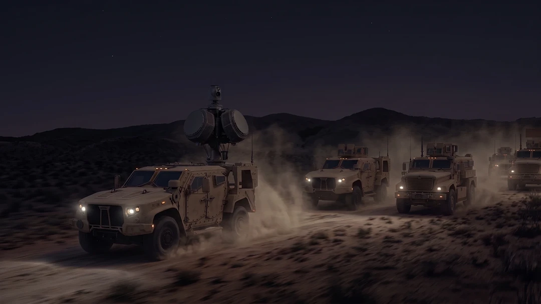
High-Precision Navigation at Scale for Counter Drone Technology
Unlock precision for your kinetic effector on-the-move. Discover how Advanced Navigation delivers the stabilization and supply chain speed needed for scalable counter drone defense.
18 May 2026
Go to Article
Navigating the Future of Mining Operations
Discover how to improve product quality in manufacturing through Advanced Navigation's rigorous supply chain and exhaustive validation.
5 May 2026
Go to Article