Laser Velocity Sensor (LVS): A High-Accuracy Velocity Aid for GNSS-Denied Navigation

Authored by: Dr. David McManus, Patrick Wiltshire, Mark Gibson, Dr. Lyle Roberts

Summary

The Laser Velocity Sensor (LVS) is a new class of navigation technology developed by Advanced Navigation that uses infrared (IR) lasers to measure a vehicle’s ground-relative 3D velocity with extraordinary accuracy and precision. To evaluate the performance of the technology, a pre-production LVS unit was integrated with an Advanced Navigation Boreas D90 fiber-optic gyroscope (FOG) inertial navigation system (INS) to demonstrate navigation in GNSS-denied conditions. A series of seven test drives were performed, with an average error per distance traveled of 0.053% compared to a GNSS reference. LVS was also tested on a fixed-wing aircraft combined with a tactical-grade INS, demonstrating a final error per distance traveled of 0.045% over the course of a 545 km flight. These results demonstrate LVS’ impressive ability to improve navigation performance in GNSS-denied or contested scenarios.

Introduction

Accurate and resilient navigation is crucial in fields such as automation, aerospace and defense. While Global Navigation Satellite Systems (GNSS) provide precise positioning and timing, they are vulnerable to signal degradation, jamming, and spoofing. Jamming disrupts GNSS signals by overpowering them with noise, while spoofing involves transmitting counterfeit signals to deceive a receiver about its true position and time ^[1][2]. The relative ease with which GNSS can be denied—whether through electronic warfare, environmental interference (e.g., physical obstruction, urban canyons) or nefarious intent—has driven demand for assured positioning, navigation, and timing (APNT) solutions.

To provide reliable navigation in GNSS-denied and contested environments, APNT technologies integrate multiple sensors for robust state estimation. At the core of these navigation systems are inertial sensors, specifically three-axis accelerometers and three-axis gyroscopes which are collectively referred to as an inertial measurement unit (IMU) ^[1]. An Inertial Navigation System (INS) consists of an IMU and a processor that integrates the IMU data to compute position and attitude. Unfortunately, errors due to sensor noise, non-linearity, and bias cause navigation solutions to diverge from the truth over time ^[3]. To mitigate this, inertial navigation systems are often aided by external velocity and position updates, such as GNSS. When GNSS is unavailable, other sensors including magnetometers, barometers, and cameras can be used to provide the INS with additional state estimates (e.g., heading, altitude, and velocity) to improve navigation performance ^{[1] [4]}.

Several APNT technologies complement INS, each offering distinct advantages and limitations depending on the application and environment:

• Visual-Inertial Odometry (VIO), which uses cameras and IMU data to estimate motion through feature tracking, is effective in structured environments but sensitive to lighting conditions and feature availability ^[5].
• Doppler Radars, which measure relative ground speed using microwave frequency Doppler shifts, and are commonly used in aircraft and military applications ^[6].
• Wheel Speed Sensors, which measure the forward velocity for ground vehicles, but require continuous ground contact and are subject to wheel slip ^[1].
• Map-Matching Techniques, which compare observed sensor data with pre-existing maps to estimate position. These can include:
  • Image-Based Visual Map Matching, which uses camera imagery to identify known landmarks ^[1].
  • Magnetic Map Matching (MagNav), which uses precise magnetometers to compare local magnetic anomalies with geomagnetic survey maps ^[7][8].
  • Gravity Map Matching (GravNav), which uses high-precision gravimeters or gravity gradiometers to align position estimates with known gravitational variations ^[9].
  • Terrain Contour Matching (TERCOM), which is commonly used in long-range autonomous platforms and aircraft, and works by comparing measured altitude profiles with digital elevation maps (DEMs) to determine position ^[10][11].
• Low Earth Orbit (LEO) Satellite Navigation, which leverages signals from commercial and government LEO constellations, and may provide greater resilience to jamming and spoofing due to their higher signal strength and diverse signal sources ^[12].

Laser Velocity Sensor (LVS)

To enhance GNSS-denied navigation capabilities, Advanced Navigation has developed the Laser Velocity Sensor (LVS)—a technology designed for precise and accurate velocity-aiding. LVS measures 3D velocity using laser Doppler velocimetry, offering exceptional accuracy and long-term stability compared to other sensors. Unlike conventional velocity sensors, LVS operates effectively on both ground and airborne platforms, provided it has a clear line of sight to the ground or another stationary surface.

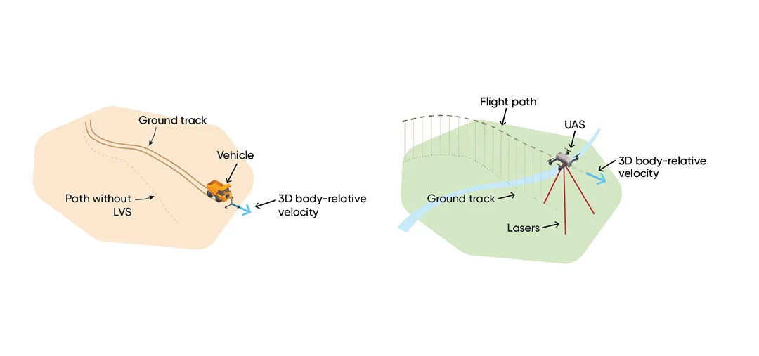
Figure 1: LVS uses lasers to measure 3D body velocity with high accuracy, and can be used in both ground and airborne applications. Measurements from LVS can be combined with an INS to provide reliable navigation even when GNSS is unreliable or unavailable.

LVS is a terrestrial adaptation of LUNA (Laser Unit for Navigation Aid), a space-grade navigation technology originally developed for autonomous lunar landings. LUNA enables reliable navigation in the harsh environment of space by providing precise three-dimensional velocity and altitude information relative to the Moon’s surface. The result of several years of R&D, LUNA is set to be demonstrated aboard Intuitive Machines’ Nova-C lander as part of NASA’s Commercial Lunar Payload Services (CLPS) program. By leveraging the engineering insights gained from LUNA, LVS transforms space technology into an Earth-ready solution for GNSS-denied navigation.

Beyond its role as a velocity aid, LVS also enhances navigation resilience by detecting GNSS spoofing. By comparing its independent velocity measurements against GNSS-derived velocity, LVS adds an extra layer of security to Assured Positioning, Navigation, and Timing (APNT) strategies. When integrated with an Inertial Navigation System (INS), such as Advanced Navigation’s high end commercial fiber optic gyroscope, the Boreas D90, LVS significantly improves navigation performance. Demonstrations with a pre-production LVS device integrated with the Boreas D90—featuring Advanced Navigation’s next-generation navigation filter—showed GNSS-denied navigation performance with an error of approximately 0.05% relative to the total distance traveled.

Principles of Operation

Doppler Velocimetry

LVS exploits the relativistic Doppler effect to estimate velocity with extraordinary precision. The principle is straightforward: when a laser beam is reflected from a surface, its frequency shifts in proportion to the velocity of the sensor relative to that surface. The magnitude of this frequency shift, Δf, is given by ^[14]

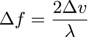
(1)

where Δf is the change in frequency due to the Doppler effect, Δv is the relative velocity between the emitter and target, and λ is the wavelength. The factor of 2 in Equation (1) is due to the fact that the laser wave experiences a Doppler frequency shift when it is reflected, and then again when it is detected.

Equation (1) highlights a key advantage of LVS over Doppler radar: the use of lasers, which operate at much shorter wavelengths (higher frequencies). For comparison, C-band lasers, with a carrier frequency of 200 THz, are 10,000 times more sensitive than K-band radar, which operates at around 20 GHz. With velocity accuracy on the order of 10 mm/s and millimetre-per-second precision, LVS significantly outperforms conventional velocity sensors. While all velocity measurements inherently contain some noise, LVS dramatically reduces the drift that limits the performance of traditional inertial navigation solutions.

Terrain Independent

LVS is suitable for use over most types of terrain, including sand, dirt, rock, grass, tree canopies, roads, and buildings. It can handle both rough and smooth surfaces, as well as hills and undulating terrain. Changes in terrain height and shape do not affect LVS, as it measures only true relativistic Doppler shifts. This ensures that LVS maintains its sensitivity when travelling up and down slopes or flying over trees, hills, and buildings.

3D Velocity Vector

LVS uses multiple laser beams in a fixed orientation relative to each other to measure the line-of-sight velocity along different vectors. Crucially, these lasers are non-scanning. To reconstruct the 3D velocity vector of the vehicle, at least three linearly independent velocity measurements are required.

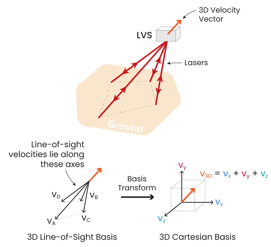
Figure 2: LVS measures the vehicle velocity along the axis of each laser beam. A basis transformation is then used to convert these ‘line-of-sight’ measurements into a 3D body velocity vector.

A basis transformation is used to convert measured line-of-sight velocities into a 3D body-frame velocity vector in a Cartesian basis (i.e., in X, Y, and Z). Accurate knowledge of the relative orientations of the line-of-sight laser vectors is required to construct the matrix used for this transformation. In the case of three emitted beams, this transformation can be expressed as

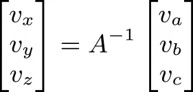
(2)

where v_a, v_b and v_c are the line-of-sight velocity measurements, A^-1 is the transformation matrix defined by the known beam orientations, and v_x, v_y and v_z represent the individual components of the 3D body-relative velocity in the Cartesian basis.

The transformation matrix A can be constructed using unit vectors â, b̂ and ĉ aligned along each of the laser beams:

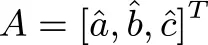
(3)

If more than three beams are emitted, this matrix can be expanded accordingly. 

An example of LVS velocity data is included in Figure 3, which shows the relationship between the three line-of-sight velocity measurements and the resulting 3D body-relative velocity components after the basis transformation.

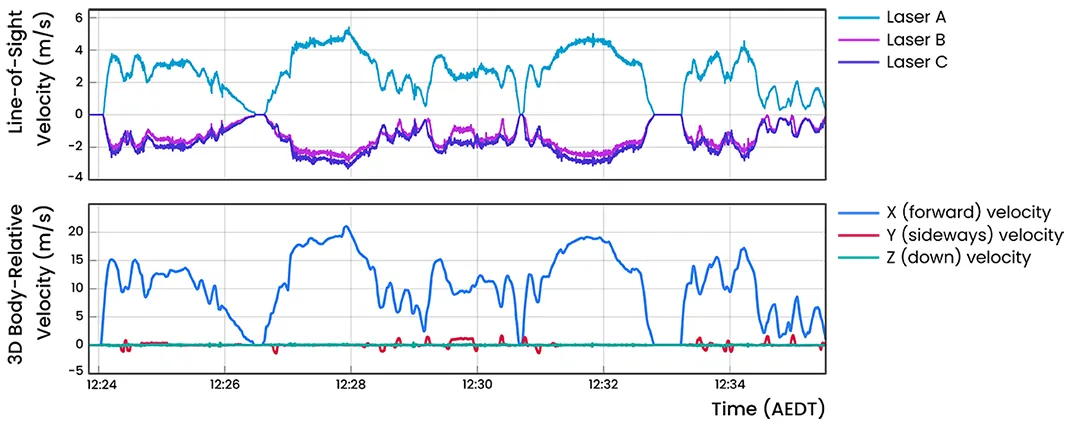
Figure 3: Time-series trace from recorded data showing the transformation from line-of-sight velocities (upper) to 3D body-relative Cartesian velocities (lower). LVS is precise enough to accurately measure sideways velocity (red in the lower trace) while the vehicle is turning, which occurs because the LVS is not at the vehicle’s centre of rotation. Advanced Navigation’s next-generation navigation filter can use these velocities to further improve bias estimation to mitigate INS drift.

An illustration of the LVS’ laser alignment is shown in Figure 4. Forward motion results in a positive Doppler shift, and thus positive line-of-sight velocity, for Laser A, whereas Lasers B and C measure negative Doppler shifts as they are pointing away from the direction of motion.

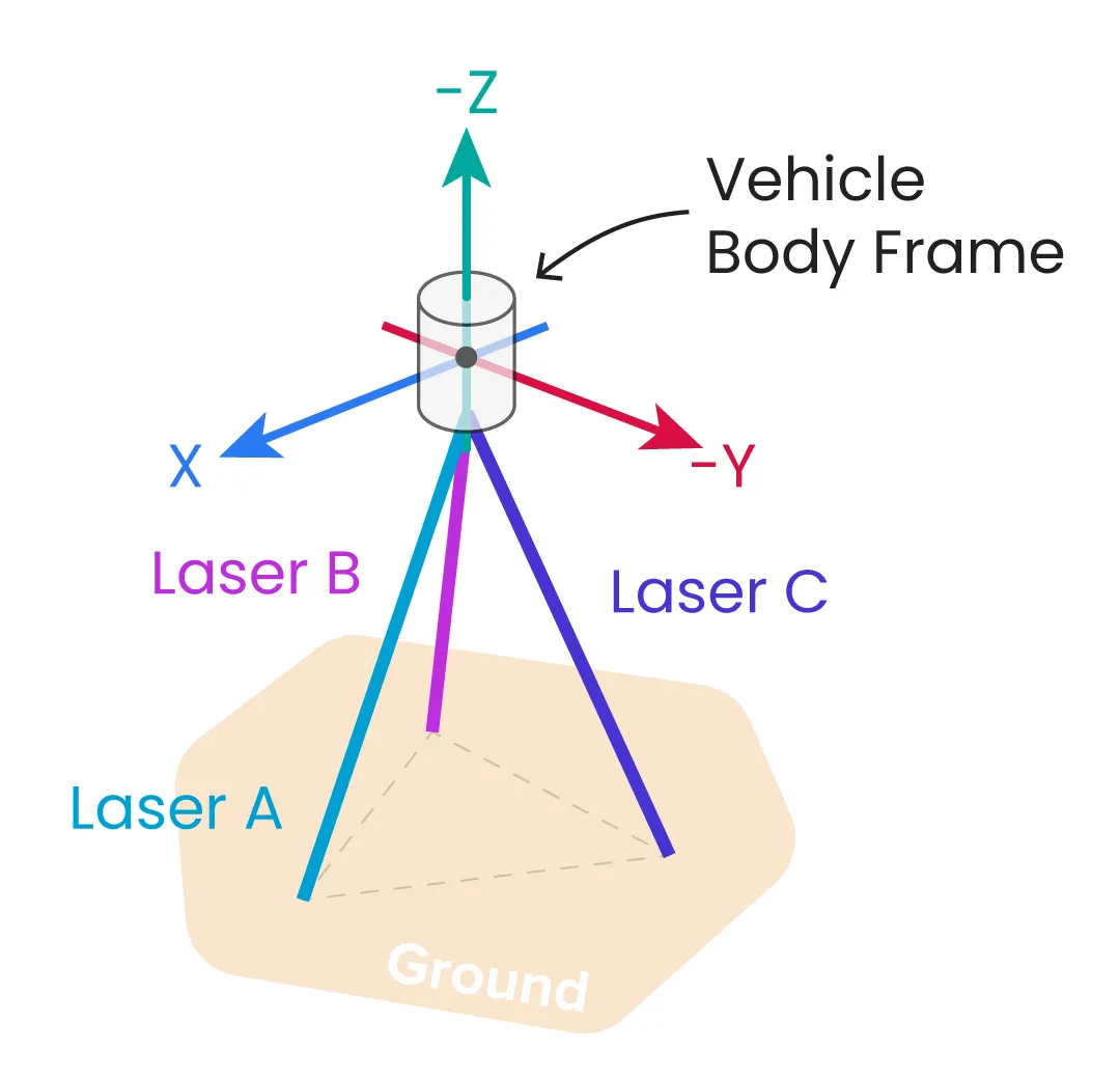
Figure 4: Orientation of the three lasers (A, B, and C) shown in Figure 3 relative to the vehicle’s 3D Cartesian body-frame.

Integration with Inertial Navigation Systems

LVS produces velocity measurements in the sensor’s body frame. To be used in navigation, these values must be transformed into a global reference frame. This requires knowledge of the vehicle’s:

1. Attitude (heading, pitch, and roll); and
2. Initial position (latitude and longitude)

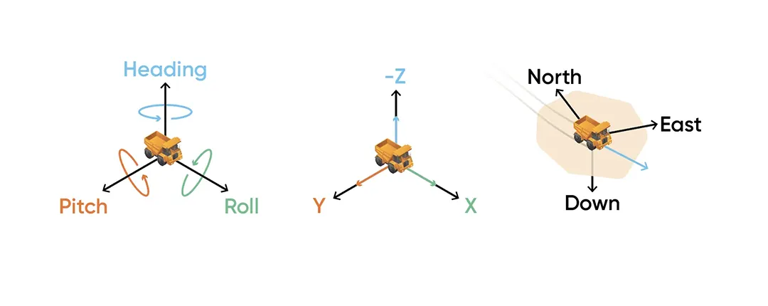
Figure 5: An Inertial Navigation System estimates how the vehicle is oriented in the global frame (heading, roll and pitch), while LVS measures relative motion in the body-frame of the vehicle. This information can be combined to estimate the vehicle’s position in the global frame.

Accurate alignment between the LVS and INS reference frames is critical. Misalignment can lead to errors in velocity translation from the body frame to the global frame ^[1]. Automatic alignment is possible when a high-accuracy reference position is available, such as GNSS with RTK or PPK corrections. Tight integration between the LVS and INS using accurate mounting guides can also be used to align the two sensors if auto-alignment using GNSS is impractical.

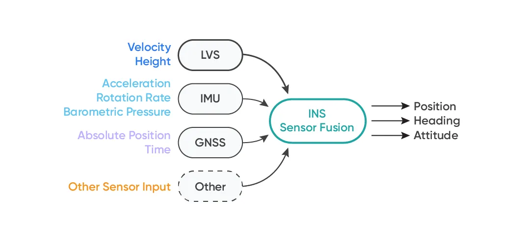
Figure 6: An Inertial Navigation System (INS) continuously estimates a vehicle’s state by fusing data from multiple sensors. Advanced Navigation’s next-generation navigation filter excels at this sensor fusion, leveraging high-precision inputs from LVS and the Boreas D90 fiber-optic gyroscopes to deliver exceptional performance, even in dynamic operating conditions.

Similar to other navigation sensors, LVS performance can be impacted by scale factor errors (e.g., due to uncertainty in the orientation of its lasers or the laser’s operating frequency). Fortunately, precise calibration and compensation techniques ensure scale factor errors remain below 100 ppm (0.01%).

Ground Vehicle Verification

To test the performance of LVS in a GNSS-denied environment, a series of controlled field demonstrations were conducted using a pre-production LVS unit integrated with an Advanced Navigation Boreas D90 INS. The test campaign involved a series of drives around Canberra designed to evaluate the LVS’ performance, consistency, and reliability.

Test Configuration

All ground vehicle tests were performed using a Tesla Model Y. The Boreas D90 INS was secured into the “frunk” (front trunk) of the vehicle alongside the LVS “sensor body”. A single GNSS antenna was mounted to the top of the vehicle using a suction mount to be used as a reference. The LVS “sensor head” was mounted to the front of the vehicle using a custom-made mount to provide line-of-sight access to the road surface in front of the vehicle. The LVS sensor body connects to the sensor head using optical fibers. The sensor head is electronically passive, and emits less than 3 mW of infrared laser light out of three different apertures. The LVS is eye safe (Class 1) so no safety precautions are necessary.

The LVS was connected to the Boreas D90 via Ethernet in a network configuration. All navigation data, including external 3D body-relative velocity packets sent to the INS from the LVS, are logged to non-volatile memory on the Boreas D90. The system was powered using a single 18 V battery. The configuration of the integrated system is shown in Figure 8.

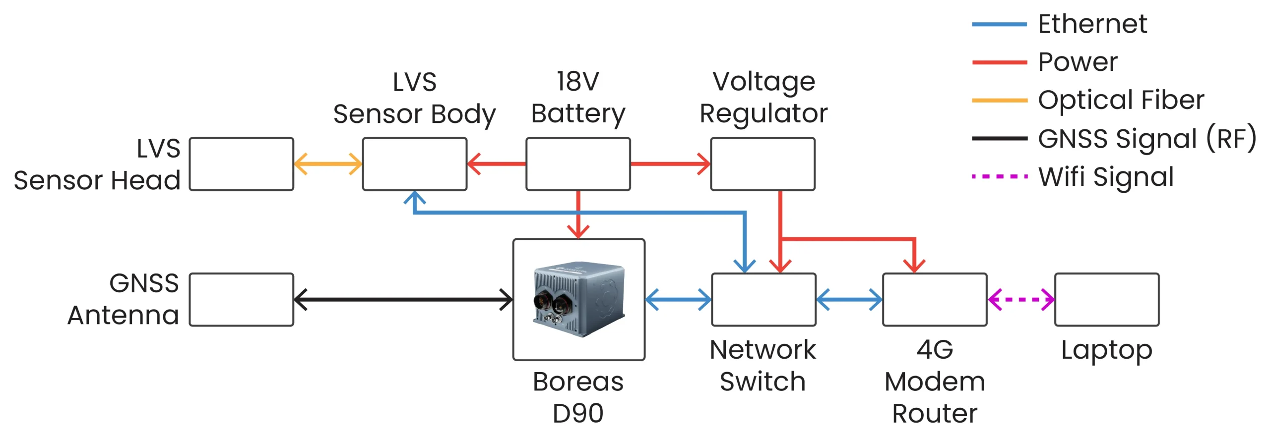
Figure 7: Configuration of the Boreas D90 FOG INS and LVS. Power was provided by a single 18V battery. Network connectivity was provided using a Network Switch and 4G Modem Router. The LVS Sensor Head and single GNSS Antenna were mounted on the vehicle’. A photograph of the system mounted in the front of the vehicle is shown in Figure 8.

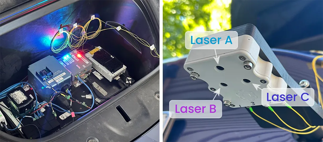
Figure 8: Configuration of the Boreas D90 INS integrated with LVS in the front of the Tesla Model Y used for ground vehicle testing. The LVS Sensor Head uses three lasers, labelled A, B, and C in the same configuration as what is shown in Figure 4.

INS Alignment

A poorly configured INS can severely degrade navigation performance in the field. Two important parameters that must be configured are a) GNSS antenna offsets, and b) the LVS Sensor Head offsets relative to the inertial frame of the INS. The spatial offsets between the INS’ reference frame, GNSS antenna, and LVS Sensor Head were measured with an estimated accuracy of 10 mm. In the case of LVS, it is also necessary to take into account the relative orientation (roll, pitch, and yaw) of the Sensor Head relative to the INS. This is extremely difficult to estimate in-situ. As such, the relative orientation was estimated using data collected from a ‘shakedown’ test. Auto-alignment of these parameters is possible using a combination of RTK GNSS and raw INS and LVS sensor data. LVS’ pitch, roll, and yaw alignment offsets were automatically calculated based on a single shakedown drive with an accuracy of 0.01º. The LVS’ initial alignment was updated once throughout testing because of suspected displacement of the LVS Sensor Head, which may have been knocked at some point during the week-long campaign.

INS Initialisation

INS initialisation is crucial, especially when being used to navigate via “dead-reckoning” (i.e., without any reliance on GNSS and with a velocity aid). In environments where access to GNSS is available, it is possible to initialise the INS’ position and heading using GNSS-derived velocity and position. Without GNSS or some other absolute position reference (e.g., map matching), it is necessary to manually initialise the INS’ position (latitude and longitude) and heading.

For the series of tests presented here, the Boreas D90 was manually reset whilst the vehicle was stationary, clearing any historical bias estimation, position, or heading information from previous tests. Immediately following the reset, Boreas D90’s position was initialised using its Primary GNSS receiver with Real Time Kinematic (RTK) corrections. Whilst stationary, Boreas’ inertial filter estimates true heading using a technique called gyrocompassing, which uses high-precision gyroscopes (e.g., fiber-optic gyroscopes and ring laser gyroscopes) to sense Earth’s rotation to determine true north. Alternatively, initial heading may be estimated using a magnetic compass or star tracker, although local environmental conditions can limit the accuracy of these devices.

Test Methodology

Seven independent tests were conducted on a ground vehicle to assess navigation performance using an Advanced Navigation pre-production LVS integrated with a Boreas D90 INS. At the start of each test, the Boreas D90 received RTK GNSS corrections to allow bias convergence. Once the heading standard deviation dropped below 0.05°, the vehicle was driven to the designated starting position.

At the start point, GNSS was disabled in the state estimation process by deselecting the Internal GNSS Enabled option in the Boreas Manager, forcing the system into dead-reckoning mode. The vehicle then completed a predefined route. Upon reaching the intended endpoint, a new Boreas log was created, and the test log was saved off-device for analysis.

Metrics for Evaluating Dead-Reckoning Performance

In each test, RTK GNSS was logged separately as a reference but was not used by the navigation filter. This approach allows for a direct comparison between the computed dead-reckoning solution and a trusted position reference. Typical GNSS accuracies vary widely: high-precision RTK GNSS achieves errors as low as 10–20 mm, while dual-band GNSS receivers (L1/L5 or L2/L5) offer 1–2 meter accuracy, and single-band receivers (L1) can exhibit errors between 2 and 10 meters ^[15]. These benchmarks highlight the expected position accuracy even when GNSS updates are available. The use of high quality RTK GNSS allows for the most accurate evaluation of the system’s dead-reckoning performance.

To facilitate this comparison, position outputs—initially given in latitude and longitude—were transformed into the North-East-Down (NED) frame, where position is expressed in meters rather than degrees, minutes, and seconds. Root-Mean-Squared Error (RMSE) is calculated by Equation 4:

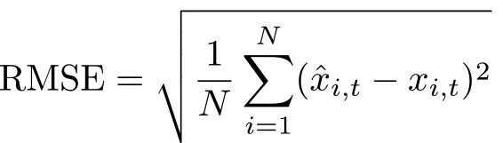
(4)

Where xi,t is denoted as the RTK GNSS position and x̂i,t  the estimated position at time t and ith test repetition. The total number of tests is given by N.

For a single test, a simplified form of RMSE, known as Root-Squared-Error (RSE), is used. Unlike RMSE, which provides an average error over all time steps, RSE gives the root squared error at each individual time step. The formula for RSE is given by Equation 5:

(5)

RMSE indicates the total error, but does not provide a measure of performance relative to the distance traveled. When dead-reckoning, small sensor errors accumulate, leading to drift in position estimates over time. To quantify this drift, position error as a percentage of distance traveled (EPD) is commonly used, calculated by Equation 6,

(6)

where Distance_t is the total path length covered by the system. This metric normalizes the error relative to the journey length, making it useful for comparing different INS configurations and sensor qualities. A lower percentage error indicates better system performance, particularly in long-duration tests where drift accumulation is a primary concern.

Test 1: GNSS-Denied Navigation, Point-to-Point

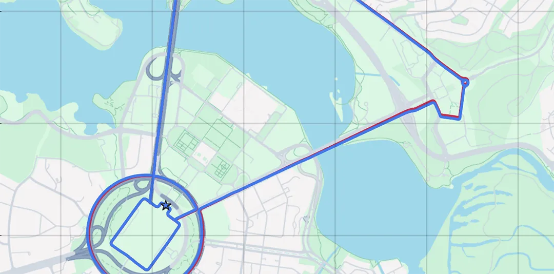
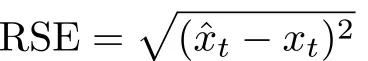
The first test completed was a longer driving test starting and finishing at different locations using LVS and Boreas D90 with GNSS-denied operation. This drive, shown in Figure 9, included fast highway speeds as well as slower driving, stopping, regular turning, and roundabouts around the suburbs of Canberra. The 23 km drive took 45 minutes and 57 seconds to complete, with a final recorded error of 4.6 m compared to the GNSS reference track. This corresponds to an error per distance traveled of 0.02%.

Figure 9: Dead-reckoning results from a 23 km drive around Canberra. GNSS was not used at any point in the drive for heading or position. RTK GNSS is shown as the red line, while the LVS + Boreas D90 navigation result is shown in blue.

Figure 10: INS position root squared error vs distance traveled for the point-to-point dead-reckoning test with a Boreas D90 and LVS. An error spike can be seen at the 9 km mark as the vehicle loses GNSS reference through a tunnel.

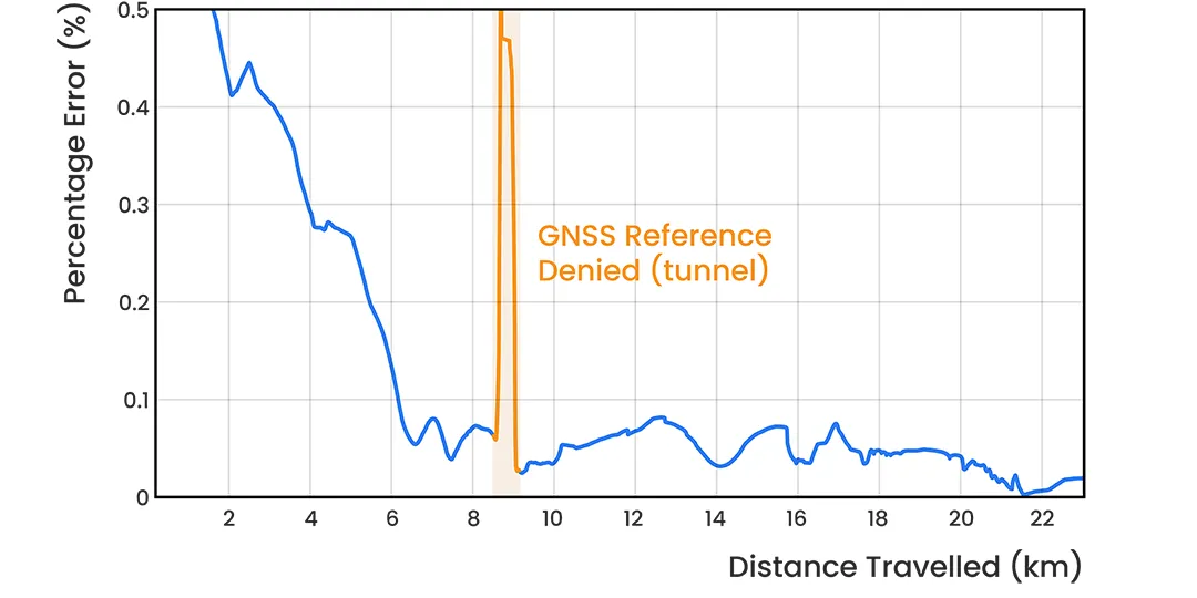
Figure 11: INS position error as a percentage of distance traveled for the point-to-point  dead-reckoning test with a Boreas D90 and LVS. An error spike can be seen at the 9 km mark as the vehicle loses GNSS reference through a tunnel.

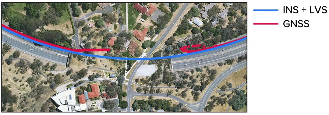
Figure 12: Zoomed section from the point-to-point GNSS-denied navigation test showing GNSS (red) drop out as the test vehicle drives through a tunnel. The LVS + Boreas navigation result can be seen in blue.

An interesting feature of this drive is the error spike seen at approximately the 9 km mark in Figures 10 and 11. This occurred when the vehicle drove through a tunnel, which completely denied the GNSS reference measurement.  Associated errors when GNSS was regained after the tunnel were due to multipath. From Figure 12, the INS + LVS trace does not suffer from this error. Position error is consistent across the drive as visible in Figure 10, which yields a decreased percentage error over distance traveled as seen in Figure 11.

Test 2: GNSS-Denied Navigation, Circuit

This test consisted of a circuit around the Parliamentary Triangle using LVS and Boreas D90 with GNSS-denied operation. This circuit includes long straight sections with faster driving as well as slower driving, stopping, turning and roundabouts. The 19.2 km circuit took 35 minutes and 15 seconds to complete, with a final recorded error of 3.5 m compared to the GNSS reference track. This corresponds to an impressive error per distance traveled of only 0.018%. As can be seen from the satellite image in Figure 13, at the end of this 19.2 km journey the vehicle is still located in the same road lane.

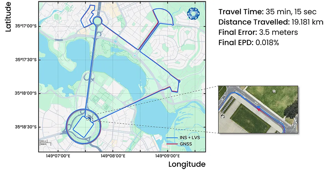
Figure 13: Navigation results from a 19.2 km drive around the Parliamentary Triangle in Canberra. GNSS was not used at any point in the drive for heading or position. RTK GNSS is shown as the red line, while the LVS + Boreas navigation result is shown in blue.

From Figure 14, it is evident that the maximum position error of 18 m occurred at approximately 9 km into the test. At the 9 km mark, the test vehicle had to navigate the myriad of construction zones around the London Circuit area due to the new phase of the Canberra light rail. Figure 15 displays the evolution of position error over distance traveled, where spikes in position RSE result in spikes in EPD.

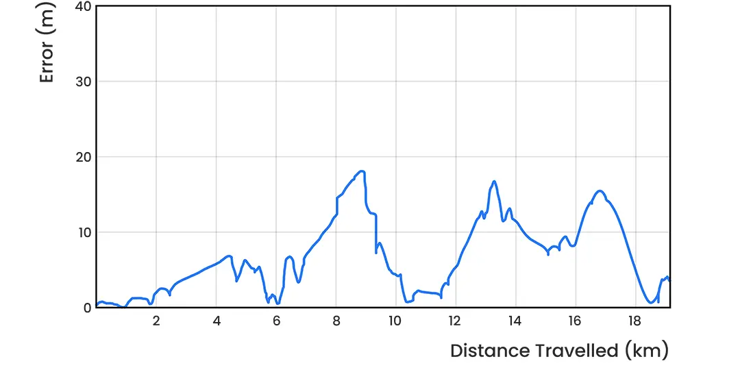
Figure 14: INS position root squared error vs distance traveled for the Parliamentary Triangle dead-reckoning test with a Boreas D90 and LVS.

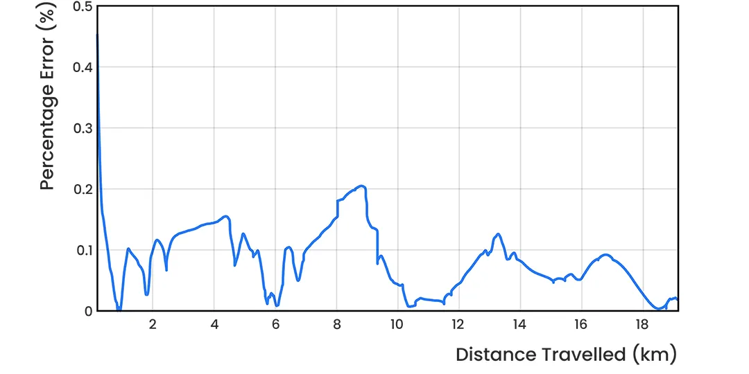
Figure 15: INS position error as a percentage of distance traveled for the Parliamentary Triangle dead-reckoning test with a Boreas D90 and LVS.

Test 3: Repeat Circuits

In order to evaluate the consistency of the system’s navigation performance, a pre-defined circuit was repeated five times. This is important because dead-reckoning performance is often cited as a “one-off” result. In order to reveal typical behaviour and performance of the technology, a number of repeat tests must be completed, controlling as many variables as possible. Traffic conditions varied during the five tests, which affected both the velocity and timing of the drive. This is expected to influence the performance and consistency of the navigation system. Sensitivity to correct alignment is further demonstrated in these repeat circuits. A sensor realignment was performed after the third drive because of a suspected disturbance to the optical head. The circuit is shown in Figure 16.

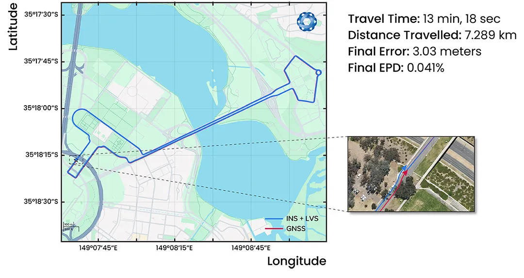
Figure 16: Navigation result from Test 5, a 7.3 km circuit around Canberra. GNSS was not used at any point in the drive for heading or position. RTK GNSS is shown in red. This same driving path was repeated five times.

The results demonstrate a high level of accuracy and consistency in position estimation. Within drives 1-3, EPD averaged 0.082%, corresponding to a mean position error of 5.91 m. After the realignment, drives 4-5 exhibited even greater accuracy, averaging 0.048% error and achieving a lower mean position error of 3.44 m, further demonstrating the system’s reliability. Across all tests, position error remained low, with an overall mean of 4.92 m and a standard deviation of just 1.79 m, highlighting stable performance. The propagation of position error over distance traveled can be seen in Figure 17.

The error metrics from these tests are included in Table 2, showing a consistently low ending EPD of 0.065% and minimal RMSE variation across tests. Drives 4-5 delivered the best results, with a final error of 0.048%, while even the highest observed errors in tests 2-3 remained below 0.105%, demonstrating strong system robustness. The low standard deviation across all tests suggests stable error propagation, ensuring repeatable and predictable dead-reckoning performance.

Table 1: Position Error Metrics for 5 Repeat Tests

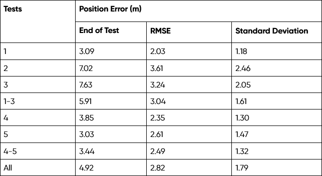
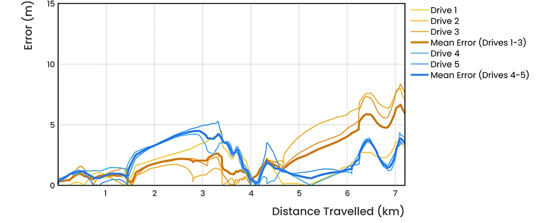
Figure 17: INS position root squared error vs distance traveled for the 5 repeat circuits dead-reckoning with a Boreas D90 and LVS.

Table 2: Position Error as a Percentage of Distance Traveled for 5 Repeat Tests

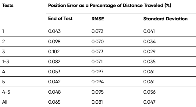
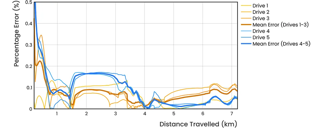
Figure 19: INS position error as a percentage of distance traveled for the 5 repeat circuits dead-reckoning with a Boreas D90 and LVS.

Airborne Vehicle Verification

To verify the performance of LVS for airborne applications, a flight test was conducted from Jandakot Airport in Western Australia using a pre-production LVS unit mounted inside a small fixed-wing aircraft.

Jandakot Flight Test

For the Jandakot flight test, an LVS unit was installed inside a Mooney 201 aircraft. A custom-designed optical head was mounted through a hole in the bottom of the craft, as shown in Figure 20. The flight covered a distance of approximately 545 km, starting and finishing at Jandakot Airport in Western Australia, with a total duration of 2 hours and 46 minutes. The aircraft took off on runway 06R and landed on runway 06L. 

During the test, the aircraft flew several long, straight sections at the same altitude, with a tight U-turn at each end. These straight sections followed the same path, as seen on the right side of Figure 21.

The highest altitude reached during the flight was 1,067 m (3500 ft). To enable the LVS to function at this altitude, the system used an optical amplifier and larger telescopes to extend its maximum range. In post-processing, the LVS velocity measurements were combined with the aircraft’s attitude vector, obtained from the onboard INS, to produce the result shown in Figure 21. This result was then compared with the GNSS trace, which was logged separately as a reference.

No GNSS position updates were used for this navigation calculation, however the heading provided by the onboard INS was aided by GNSS, which helped eliminate the effects of INS heading drift on the final result.

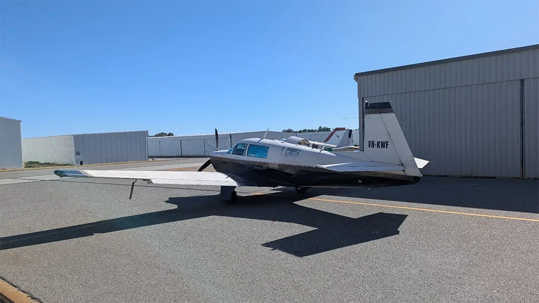
Figure 20: The Mooney 201 that was used for the Jandakot flight test. A custom optical head was mounted inside of the plane with lasers emitted through a hole in the bottom.

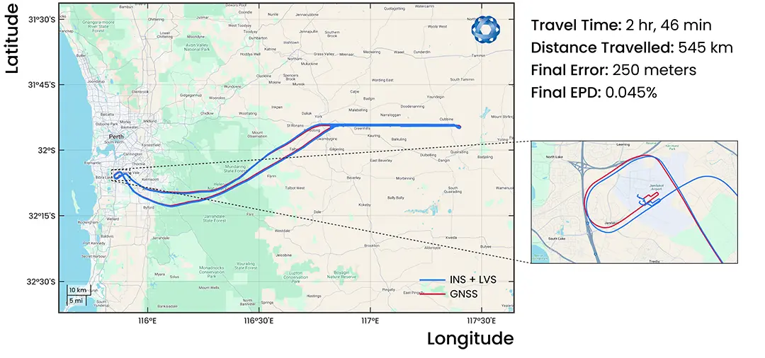
Figure 21: Navigation results from a 545 km flight starting and ending at Jandakot Airport. GNSS position was not used to update the LVS result. The heading of the aircraft as reported by the on board INS was influenced by GNSS, which removes the effect of heading drift from this result. The cut-out image on the right shows a zoomed in version of the start and finish of the run RTK GNSS is shown as the red line, while the LVS + Boreas navigation result is shown in blue. The aircraft took off on runway 06R and landed on runway 06L. The accumulated error in the INS + LVS track coincidentally lines up with runway 06R.

The final error following the 545 km flight was 250 m, corresponding to an error per distance traveled of 0.05%. The maximum error in the flight was 900 m, which occurred during the first of the three hairpin manoeuvres performed during the flight. Figure 22 shows the error between the LVS navigation result and the GNSS reference at different distances throughout the flight. Figure 23 shows this error as a percentage of the distance traveled.

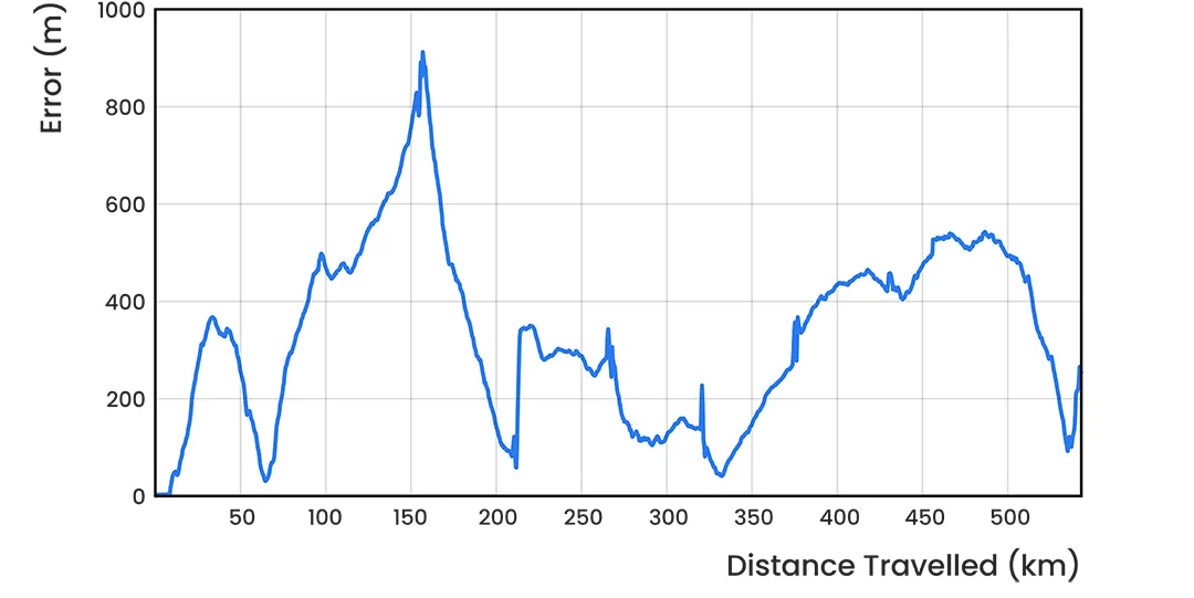
Figure 22: INS root squared position error against distance traveled on the Mooney 201 light aircraft using dual antenna GNSS heading and integrating LVS data.

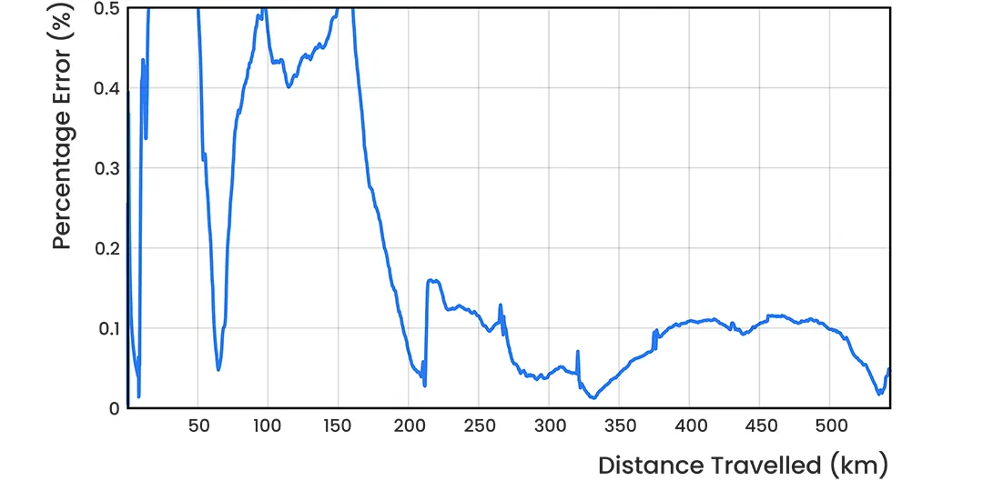
Figure 23: INS position error as a percentage of distance traveled on the Mooney 201 light aircraft using dual antenna GNSS heading and integrating LVS data.

Conclusion

LVS is a precision 3D velocity sensor that can be combined with a high performance INS such as an Advanced Navigation Boreas D90 to achieve exceptional navigation performance even in fully GNSS-denied environments. LVS and Boreas were used in multiple ground vehicle tests, achieving an average error per distance traveled of 0.0526% over seven test drives in fully GNSS-denied conditions. LVS was also tested on a fixed-wing aircraft and was combined with a tactical grade INS to achieve an error per distance traveled of 0.05% during a 545 km flight.

Acknowledgements

We would like to express our sincere gratitude to Transparent Earth Geophysics (TEG) for their invaluable support in conducting our flight testing. As experts in airborne geophysics, TEG provide access to world-class pilots and aircraft, enabling us to rigorously test and refine our technology. Through our close collaboration with the TEG team, we have been able to perform regular—almost routine—flight tests out of Jandakot Airport in Western Australia, significantly advancing our development efforts.

References

1 Groves, Paul D.(2013). Principles of GNSS, Inertial, and Multisensor Integrated Navigation Systems, Second Edition (GNSS Technology and Applications) Artech House. ISBN 978-1608070053. 

2 Meng, Lianxiao, Lin Yang, Wu Yang, and Long Zhang. 2022. “A Survey of GNSS Spoofing and Anti-Spoofing Technology” Remote Sensing 14, no. 19: 4826. https://doi.org/10.3390/rs14194826

3 Woodman, O.J. An introduction to inertial navigation. Technical report, University of Cambridge, Computer Laboratory, 2007.

4 Chow, J. C. Statistical sensor fusion of a 9-dof mems imu for indoor navigation. arXiv preprint arXiv:1802.04388, 2018.

5 Bonin-Font, Francisco & Ortiz, Alberto & Oliver, Gabriel. (2008). Visual Navigation for Mobile Robots: A Survey. Journal of Intelligent and Robotic Systems. 53. 263-296. 10.1007/s10846-008-9235-4. 

6 W. R. Fried, “Principles and Performance Analysis of Doppler Navigation Systems,” in IRE Transactions on Aeronautical and Navigational Electronics, vol. ANE-4, no. 4, pp. 176-196, Dec. 1957, doi: 10.1109/TANE3.1957.4201552.

7 A. Canciani and J. Raquet, “Airborne Magnetic Anomaly Navigation,” IEEE Transactions on Aerospace and Electronic Systems, vol. 53, no. 1, pp. 67–80, Feb. 2017, conference Name: IEEE Transactions on Aerospace and Electronic Systems. [Online]. Available: https: //ieeexplore.ieee.org/document/7808987 

8 “Absolute Positioning Using the Earth’s Magnetic Anomaly Field,” NAVIGATION, vol. 63, no. 2, pp. 111–126, 2016, eprint: https://onlinelibrary.wiley.com/doi/pdf/10.1002/navi.138. [Online]. Available: https://onlinelibrary.wiley.com/doi/abs/10.1002/navi. 138

9 Javed, Waqas & Ghani, Sohaib & Elmqvist, Niklas. (2012). GravNav: Using a Gravity Model for Multi-Scale Navigation. Proceedings of the Workshop on Advanced Visual Interfaces AVI. 10.1145/2254556.2254597. 

10 Baird, C.A., 1985. Design techniques for improved map-aided navigation. NAECON 1985, pp.231-238.

11  Hinrichs, P.R., 1976. Advanced terrain correlation techniques(position locating system in war environments). In Position Location and Navigation Symposium, San Diego, Calif (pp. 89-96).

12 Prol, Fabricio & Ferre, Ruben & Saleem, Z. & Välisuo, Petri & Pinell, C. & Lohan, Elena Simona & Elsanhoury, Mahmoud & Elmusrati, Mohammed & Islam, Saiful & Celikbilek, K. & Selvan, Kannan & Yliaho, J. & Rutledge, Kendall & Ojala, Arto & Ferranti, L. & Praks, J. & Bhuiyan, Mohammad Zahidul H. & Kaasalainen, S. & Kuusniemi, H.. (2022). Position, Navigation, and Timing (PNT) Through Low Earth Orbit (LEO) Satellites: A Survey on Current Status, Challenges, and Opportunities. IEEE Access. 10. 1-1. 10.1109/ACCESS.2022.3194050.

13 Advanced Navigation, “Boreas D90 Datasheet, v1.5, March 2025, link: https://www.advancednavigation.com/inertial-navigation-systems/fog-gnss-ins/boreas/d90-datasheet/

‌14 Walker, Jearl; Resnick, Robert; Halliday, David (2007). Halliday & Resnick Fundamentals of Physics (8th ed.). Wiley. ISBN 9781118233764. OCLC 436030602.15 Manandhar, D. (n.d.). Interpreting GNSS Specifications. [online] The University of Tokyo: Center for Spatial Information Sciences. Available at: https://www.unoosa.org/documents/pdf/icg/2021/Tokyo2021/ICG_CSISTokyo_2021_19.pdf

• FOG GNSS/INS
• INS
• Laser Velocity Sensor
• LVS
• Research and Development

Recent Tech Articles

Laser Velocity Sensor (LVS): A High-Accuracy Velocity Aid for GNSS-Denied Navigation

The Laser Velocity Sensor (LVS) is a new class of navigation technology developed by Advanced Navigation that uses infrared (IR) lasers to measure a vehicle’s ground-relative 3D velocity with extraordinary accuracy and precision.

30 March 2025

Go to Article

Inertial Navigation: Empowering Armored Combat Vehicles in GNSS-Denied Environments

With low-cost GPS jamming and spoofing technologies becoming widely available, relying solely on GPS for navigation has become an increasingly risky option for armored combat vehicles. Despite the dangers, many defense fleets around the world remain ill-equipped to navigate effectively through contested environments where GPS is compromised.

3 September 2024

Go to Article